The Bernoulli and Binomial Distributions

STA 211 · Lecture 07

Introduction

The Bernoulli distribution models a single trial with two outcomes. The Binomial distribution models the number of successes in a fixed number of independent Bernoulli trials with constant success probability.

Learning Objectives

You should be able to:

• identify Bernoulli and binomial experiments;
• derive their probability functions;
• calculate means, variances and MGFs;
• use cumulative and complementary probabilities; and
• apply the additivity property of binomial variables.

Bernoulli Distribution

Let $X = 1$ for success and $X = 0$ for failure. If $P(X = 1) = p$ and $q = 1 - p$, then

$$p_{X}(x) = p^{x}q^{1 - x},\quad\quad x = 0,1.$$

The mean and variance are

$$E(X) = p,$$

$$Var(X) = pq.$$

The MGF is

$$M_{X}(t) = q + pe^{t}.$$

Binomial Distribution

A random variable $X$ has a binomial distribution with parameters $n$ and $p$, written $X \sim Bin(n,p)$, if:

1. there are $n$ trials;
2. each trial has two outcomes;
3. trials are independent; and
4. the success probability $p$ is constant.

The PMF is

$$P(X = x) = \binom{n}{x}p^{x}q^{n - x},\quad\quad x = 0,1,\ldots,n.$$

The term $\binom{n}{x}$ counts the positions of the $x$ successes; $p^{x}q^{n - x}$ is the probability of any one such pattern.

Binomial probability mass function

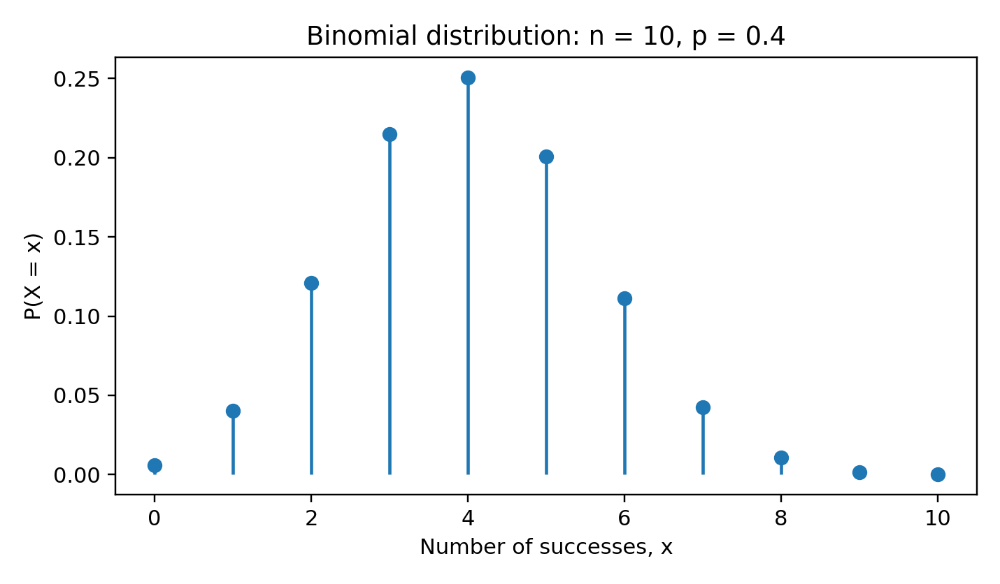
Binomial probability mass function

The mean and variance are

$$E(X) = np,$$

$$Var(X) = npq.$$

The MGF is

$$M_{X}(t) = \left( q + pe^{t} \right)^{n}.$$

Useful Probability Forms

Exactly $x$ successes:

$$P(X = x) = \binom{n}{x}p^{x}q^{n - x}.$$

At most $r$ successes:

$$P(X \leq r) = \sum_{x = 0}^{r}\binom{n}{x}p^{x}q^{n - x}.$$

At least one success:

$$P(X \geq 1) = 1 - P(X = 0) = 1 - q^{n}.$$

More than $r$ successes:

$$P(X > r) = 1 - P(X \leq r).$$

Example 7.1

A production process has a 5% defect rate. In a random sample of 10 independent items, the probability of exactly 2 defects is

$$\binom{10}{2}(0.05)^{2}(0.95)^{8} \approx 0.0746.$$

The probability of at least one defect is

$$1 - (0.95)^{10} \approx 0.4013.$$

Additivity

If $X \sim Bin\left( n_{1},p \right)$ and $Y \sim Bin\left( n_{2},p \right)$ are independent with the same success probability, then

$$X + Y \sim Bin\left( n_{1} + n_{2},p \right).$$

The same $p$ is essential. If the success probabilities differ, the sum is not generally binomial.

Recurrence Relation

Successive probabilities satisfy

$$\frac{P(X = x + 1)}{P(X = x)} = \frac{n - x}{x + 1}\frac{p}{q}.$$

This relation can reduce repetitive calculation and helps locate the mode.

Post-Test

1. State the four assumptions of a binomial model.
2. If $X \sim Bin(12,0.3)$, find $E(X)$ and $Var(X)$.
3. Find $P(X = 4)$ for the distribution in Question 2.
4. A fair coin is tossed 8 times. Find the probability of at least 6 heads.
5. Explain when the sum of two independent binomial variables is binomial.

Selected answers: 2. $3.6$ and $2.52$; 3. $\binom{12}{4}(0.3)^{4}(0.7)^{8} \approx 0.2311$; 4. $\sum_{x = 6}^{8}\binom{8}{x}2^{- 8} = 37/256$.

Previous lecture

Course home

Next lecture