The Normal Distribution

STA 211 · Lecture 12

Introduction

The normal distribution is central to probability and statistics because it models many approximately symmetric measurements and arises as the limiting distribution of standardised sums under broad conditions.

Learning Objectives

You should be able to:

• state the normal density and its properties;
• standardise normal variables;
• calculate probabilities using the standard normal distribution;
• use linear transformation and additivity; and
• apply a normal approximation to the binomial distribution.

Normal Density

A random variable $X$ has a normal distribution with mean $\mu$ and variance $\sigma^{2}$, written

$$X \sim N\left( \mu,\sigma^{2} \right),$$

if

$$f_{X}(x) = \frac{1}{\sigma\sqrt{2\pi}}\exp\left\lbrack - \frac{(x - \mu)^{2}}{2\sigma^{2}} \right\rbrack,\quad\quad - \infty < x < \infty.$$

Standard normal probability density function

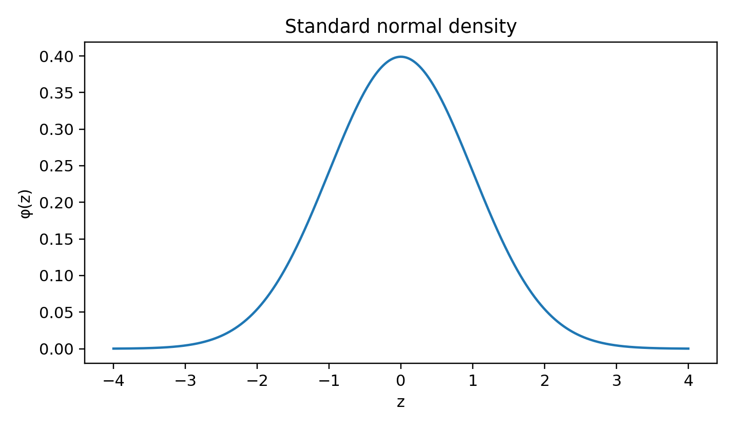
Standard normal probability density function

The density is symmetric about $\mu$, with mean, median and mode all equal to $\mu$.

Standardisation

If $X \sim N\left( \mu,\sigma^{2} \right)$, then

$$Z = \frac{X - \mu}{\sigma} \sim N(0,1).$$

Therefore,

$$P(a < X < b) = P\left( \frac{a - \mu}{\sigma} < Z < \frac{b - \mu}{\sigma} \right).$$

Let $\Phi(z) = P(Z \leq z)$ denote the standard normal CDF. Symmetry gives

$$\Phi( - z) = 1 - \Phi(z).$$

Example 12.1

Suppose examination scores are normal with mean 60 and standard deviation 8. The probability that a score exceeds 72 is

$$P(X > 72) = P\left( Z > \frac{72 - 60}{8} \right) = P(Z > 1.5).$$

Using the standard normal table,

$$P(Z > 1.5) = 1 - \Phi(1.5) \approx 0.0668.$$

MGF and Linear Transformation

The MGF is

$$M_{X}(t) = exp\left( \mu t + \frac{1}{2}\sigma^{2}t^{2} \right).$$

If $Y = a + bX$, then

$$Y \sim N\left( a + b\mu,b^{2}\sigma^{2} \right).$$

Additivity

If $X_{i} \sim N\left( \mu_{i},\sigma_{i}^{2} \right)$ are independent, then

$$\sum_{i = 1}^{n}X_{i} \sim N\left( \sum_{i = 1}^{n}\mu_{i},\sum_{i = 1}^{n}\sigma_{i}^{2} \right).$$

More generally, any linear combination of jointly normal variables is normal.

Empirical Rule

For a normal distribution, approximately:

$$P\left( |X - \mu| < \sigma \right) \approx 0.6827,$$

$$P\left( |X - \mu| < 2\sigma \right) \approx 0.9545,$$

$$P\left( |X - \mu| < 3\sigma \right) \approx 0.9973.$$

Normal Approximation to the Binomial

If $X \sim Bin(n,p)$ and both $np$ and $nq$ are sufficiently large, then

$$X \approx N(np,npq).$$

Because the binomial is discrete and the normal is continuous, use a continuity correction. For example,

$$P(X \leq x) \approx P(Y \leq x + 0.5),$$

where $Y \sim N(np,npq)$.

Example 12.2

Let $X \sim Bin(100,0.4)$. Approximate $P(X \leq 45)$.

Here $\mu = 40$ and $\sigma = \sqrt{24} \approx 4.899$. With continuity correction,

$$P(X \leq 45) \approx P\left( Z \leq \frac{45.5 - 40}{4.899} \right) = P(Z \leq 1.123) \approx 0.869.$$

Post-Test

1. State the normal PDF and standardisation formula.
2. If $X \sim N(50,100)$, find $P(X > 65)$ in terms of $\Phi$.
3. If $X \sim N(10,4)$ and $Y = 3X - 2$, state the distribution of $Y$.
4. Independent variables have distributions $N(5,4)$ and $N(2,9)$. State the distribution of their sum.
5. Explain the continuity correction in a normal approximation to the binomial.

Selected answers: 2. $1 - \Phi(1.5)$; 3. $N(28,36)$; 4. $N(7,13)$.

Previous lecture

Course home

Next lecture