The Negative Binomial and Geometric Distributions

STA 211 · Lecture 08

Introduction

The binomial model fixes the number of trials and counts successes. The negative binomial model reverses this structure: it fixes the required number of successes and counts how many trials are needed. The geometric distribution is the special case in which the first success is awaited.

Learning Objectives

You should be able to:

• identify negative binomial and geometric experiments;
• use their PMFs, means and variances;
• distinguish common support conventions; and
• explain the memoryless property of the geometric distribution.

Negative Binomial Distribution

Let $X$ be the trial on which the $r$th success occurs. For independent Bernoulli trials with success probability $p$ and $q = 1 - p$,

$$P(X = x) = \binom{x - 1}{r - 1}p^{r}q^{x - r},\quad\quad x = r,r + 1,\ldots.$$

The last trial must be a success. Among the first $x - 1$ trials, exactly $r - 1$ must be successes.

The mean and variance are

$$E(X) = \frac{r}{p},$$

$$Var(X) = \frac{rq}{p^{2}}.$$

The MGF is

$$M_{X}(t) = \left( \frac{pe^{t}}{1 - qe^{t}} \right)^{r},\quad\quad qe^{t} < 1.$$

Negative binomial probability mass function

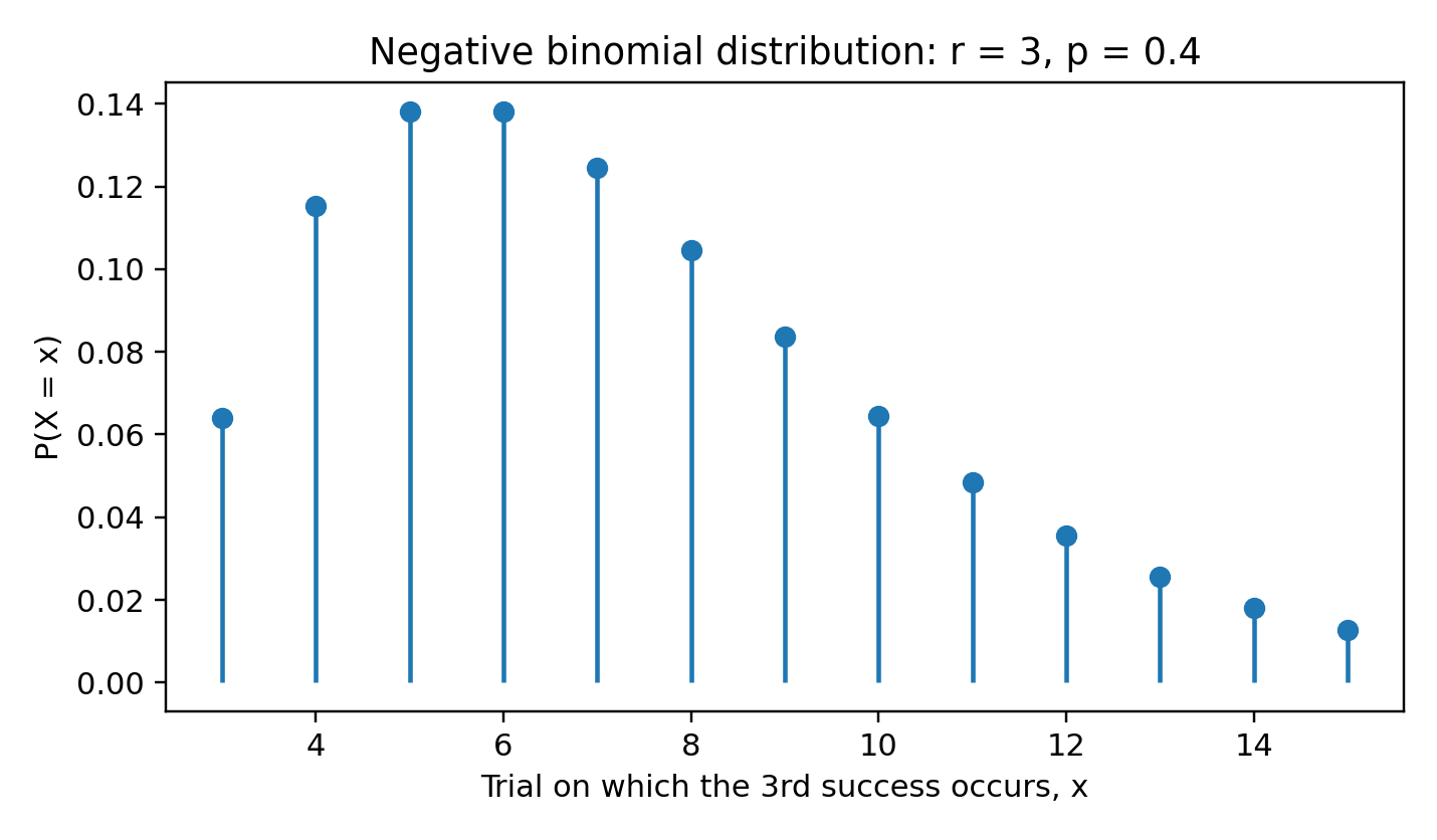
Negative binomial probability mass function

Alternative convention

Some texts define $Y = X - r$ as the number of failures before the $r$th success. Then

$$P(Y = y) = \binom{y + r - 1}{r - 1}p^{r}q^{y},\quad\quad y = 0,1,2,\ldots,$$

with

$$E(Y) = \frac{rq}{p},\quad\quad Var(Y) = \frac{rq}{p^{2}}.$$

Always state the convention before using a formula.

Geometric Distribution

For $r = 1$, $X$ is the trial of the first success:

$$P(X = x) = pq^{x - 1},\quad\quad x = 1,2,\ldots.$$

Its mean and variance are

$$E(X) = \frac{1}{p},$$

$$Var(X) = \frac{q}{p^{2}}.$$

The tail probability is

$$P(X > k) = q^{k}.$$

Memoryless Property

The geometric distribution is memoryless:

$$P(X > s + t \mid X > s) = P(X > t).$$

After $s$ failures, the waiting time distribution for the first success is unchanged because Bernoulli trials are independent and have constant success probability.

Example 8.1

A salesperson closes a sale with probability 0.25 on each independent call. The probability that the first sale occurs on the fifth call is

$$(0.75)^{4}(0.25) \approx 0.0791.$$

The expected number of calls is

$$E(X) = \frac{1}{0.25} = 4.$$

Example 8.2

If a laboratory test succeeds with probability 0.6, the probability that the third success occurs on the fifth trial is

$$\binom{4}{2}(0.6)^{3}(0.4)^{2} = 0.20736.$$

Post-Test

1. State the support of the trial-count negative binomial variable.
2. If $X$ is geometric with $p = 0.2$, find $P(X = 4)$ and $P(X > 4)$.
3. Find the mean and variance of a negative binomial variable with $r = 5$ and $p = 0.4$.
4. Explain the difference between “trials until the $r$th success” and “failures before the $r$th success”.
5. Prove the memoryless property using the tail probability.

Selected answers: 2. $0.2(0.8)^{3} = 0.1024$, $(0.8)^{4} = 0.4096$; 3. $12.5$ and $18.75$.

Previous lecture

Course home

Next lecture