The Poisson Distribution

STA 211 · Lecture 09

Introduction

The Poisson distribution models counts of events occurring randomly in a fixed interval of time, space, area or volume. It is appropriate when events occur independently at a stable average rate and simultaneous events in a very small interval are negligible.

Learning Objectives

You should be able to:

• recognise a Poisson count model;
• calculate Poisson probabilities;
• derive its mean, variance and MGF;
• explain its process assumptions and additivity; and
• use it as an approximation to the binomial distribution.

Poisson Probability Function

A random variable $X$ has a Poisson distribution with parameter $\lambda > 0$, written $X \sim Pois(\lambda)$, if

$$P(X = x) = e^{- \lambda}\frac{\lambda^{x}}{x!},\quad\quad x = 0,1,2,\ldots.$$

The parameter $\lambda$ is both the mean and variance:

$$E(X) = \lambda,$$

$$Var(X) = \lambda.$$

The MGF is

$$M_{X}(t) = exp\{\lambda\left( e^{t} - 1 \right)\}.$$

Poisson probability mass function

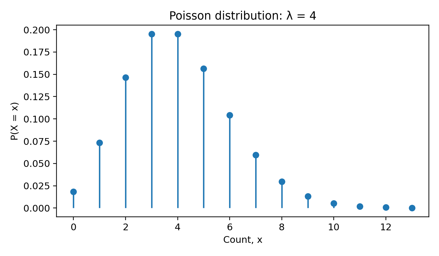
Poisson probability mass function

Poisson Process Interpretation

For a homogeneous Poisson process with rate $\rho$ per unit interval, the count in an interval of length $t$ has parameter

$$\lambda = \rho t.$$

The model assumes:

1. counts in disjoint intervals are independent;
2. the event rate is constant;
3. the probability of one event in a very short interval is approximately proportional to its length; and
4. the probability of two or more events in a very short interval is negligible relative to its length.

Example 9.1: Calls

A help desk receives an average of 4 calls per 10 minutes. The probability of exactly 6 calls in 10 minutes is

$$e^{- 4}\frac{4^{6}}{6!} \approx 0.1042.$$

The probability of no calls is

$$P(X = 0) = e^{- 4} \approx 0.0183.$$

Recurrence Relation

Successive probabilities satisfy

$$P(X = x + 1) = \frac{\lambda}{x + 1}P(X = x).$$

Additivity

If $X_{i} \sim Pois\left( \lambda_{i} \right)$ are independent, then

$$\sum_{i = 1}^{n}X_{i} \sim Pois\left( \sum_{i = 1}^{n}\lambda_{i} \right).$$

This follows immediately by multiplying their MGFs.

Poisson Limit of the Binomial

If $X_{n} \sim Bin\left( n,p_{n} \right)$, $n \rightarrow \infty$, $p_{n} \rightarrow 0$, and $np_{n} \rightarrow \lambda$, then

$$P\left( X_{n} = x \right) \rightarrow e^{- \lambda}\frac{\lambda^{x}}{x!}.$$

This justifies the approximation

$$Bin(n,p) \approx Pois(np)$$

when $n$ is large and $p$ is small. A common practical guide is $p \leq 0.05$ and $np$ not too large, though accuracy should be assessed in context.

Example 9.2: Rare defects

In 200 independent items, each has defect probability 0.01. With $\lambda = np = 2$,

$$P(X \leq 1) \approx e^{- 2}(1 + 2) = 3e^{- 2} \approx 0.4060.$$

Post-Test

1. State the Poisson PMF and support.
2. If $X \sim Pois(3)$, find $P(X = 0)$ and $P(X \geq 1)$.
3. Calls arrive at 6 per hour. Find the probability of 2 calls in 20 minutes.
4. If $X \sim Pois(2)$ and $Y \sim Pois(5)$ are independent, state the distribution of $X + Y$.
5. Approximate $P(X = 0)$ for $X \sim Bin(500,0.004)$ using a Poisson model.

Selected answers: 2. $e^{- 3}$ and $1 - e^{- 3}$; 3. with $\lambda = 2$, $P(X = 2) = 2e^{- 2}$; 4. $Pois(7)$; 5. $e^{- 2}$.

Previous lecture

Course home

Next lecture